Development of analyses for 2⁶⁰⁰⁰ variants

Many software systems provide a large number of configuration options to adapt the behavior of a system to different requirements and use cases. Such variant-rich systems pose a great challenge to the quality assurance of software systems. Due to the possible combinatorics, a “brute force” assurance of every single possible variant is not an option.

The Linux kernel, for example, offers more than 6000 configuration options. Among them options for different file systems (EXT3, EXT4, JFS, XFS, Btrfs, …), various USB devices, numerous processor types and many more. With their help, in theory, up to 2⁶⁰⁰⁰ Linux kernel variants for smartphones, routers, high-performance computers or standard PCs can be created at the push of a button. Even though the actual number of Linux kernel variants is lower due to dependencies between configuration options, it is still in an astronomically large range.

Implementing Variability with the C Preprocessor

Variability is implemented in the Linux kernel using the C preprocessor (cpp). The C preprocessor is a simple text processing tool and an essential part of software development in C (through integration with C compilers). Software developers can use so-called directives to provide specifications for text processing.

In the context of implementing variant-rich systems, developers use directives such as #ifdef to encode variable code fragments. #ifdef directives behave like normal if statements of C, except that they are evaluated by the preprocessor to compile (translate) a program. If the expressions contained in #ifdef directives (a logical combination of configuration options) evaluate to true the code fragment remains in the generated variant. Otherwise, it is removed by the preprocessor.

Let us look at the following example of a configurable function implementation in C (for presentation purposes, the preprocessor directives #ifdef and #endif are shown inline):

C-Beispiel

1int foo(int a #ifdef X, int b #endif) {
2  int c = a;
3  if (c) {
4    c = 1;
5#ifdef Y c = c+b; #endif
6  }
7  return c;
8}

The function implementation can be configured by the X and Y options. The two options control the presence or absence of two code fragments. Option Y controls the function parameter int b. Option Y controls the assignment c = c+b. Based on the values for X and Y (either true/1 or false/0) four different variants of the function can be created:

1. X = false; Y = false;
2. X = false; Y = true;
3. X = true; Y = false;
4. X = true; Y = true;

#ifdef Directives play an important role in the implementation of variability in C source code, and so #ifdef directives are used in many software systems written in C. Among them, for example:

• The database system PostgreSQL,
• The version control system Subversion (SVN),
• The cryptographic library OpenSSL,
• The text editor VIM,
• The Python programming language,
• The web server Apache,
• and many more.

The number of configuration options in these runs into the hundreds/thousands. The combinatorics of true and false for different configuration options quickly creates an astronomically large number of different variants that can be created from a single, configurable system by generation. The validation of these variants is a major challenge because, if possible, all variants should be fully validated for the delivery of the system. Errors can arise quite quickly during the development of a variant-rich system.

For example, the above example contains a type error: the variable b in the assignment c = c+b is not defined for the combination X = false and Y = true because the function parameter int b is removed by the preprocessor before compilation.

The following simple strategy could be used to check such errors: First, each possible variant is generated, to be checked afterwards by means of an analysis. However, this approach, also known in practice as brute force, does not scale because with an assumed analysis time of 10s per variant, the total time to analyze the Linux kernel with 2⁶⁰⁰⁰ variants would take 4.8*10¹⁷⁹⁹ years.

Although the individual function implementation variants are different, they share many similarities. For example, in the example, all variants share the function parameter int a (line 1) and the statement for the return value of the function return c (line 7). Thus, analysis strategies that examine individual variants analyze common components multiple times with exponential effort.

Variability-true analyses: data structures and algorithms

Variability-true analyses are a strategy to avoid redundant computations of analysis results. The strategy is based on taking variability information (i.e., dependencies in the form of #ifdefs with configuration options) into account when computing analysis results, so that both similarities and differences (i.e., variable code fragments) need to be analyzed only once.

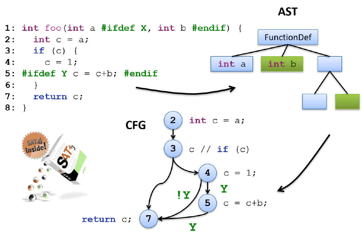
Static analyses (e.g. type checking or data flow analyses), as they are typically used in programming environments such as Eclipse or IntelliJ Idea, usually do not work directly on the source code, but use suitable representations of the source code. A typical representation is an Abstract Syntax Tree (AST). This reflects the essential structure of the program code and abstracts from the syntax (among other things, bracketing, code indentation or comments). To represent source code with #ifdef directives we use an AST tree in which variable code fragments can be represented. For example, function parameter int b is a variable node in the AST (shown here in green). The AST created in this way represents all four variants of the configurable function implementation in a compact representation.

Another representation for static analysis is the control flow graph (CFG). A CFG represents all possible execution paths in a program by a successor relationship of program instructions (successor or succ relationship). Thus, the successor of the assignment int c = a (line 2) is always the condition c of the if statement (line 3). In our context, the CFG represents the execution paths of all possible variants of the function implementation. This leads to the fact that the successor of a program statement can be a variable result and depends on configuration options. For example, program statement following c = 1 (line 4) is a variable result and depends on configuration option Y. If Y = true, then c = c+b is executed as the next instruction. With Y = false the return value of the function return c follows. This compact representation of all program execution paths is the basis for efficient calculation of analysis results for data flow analysis.

Three principles

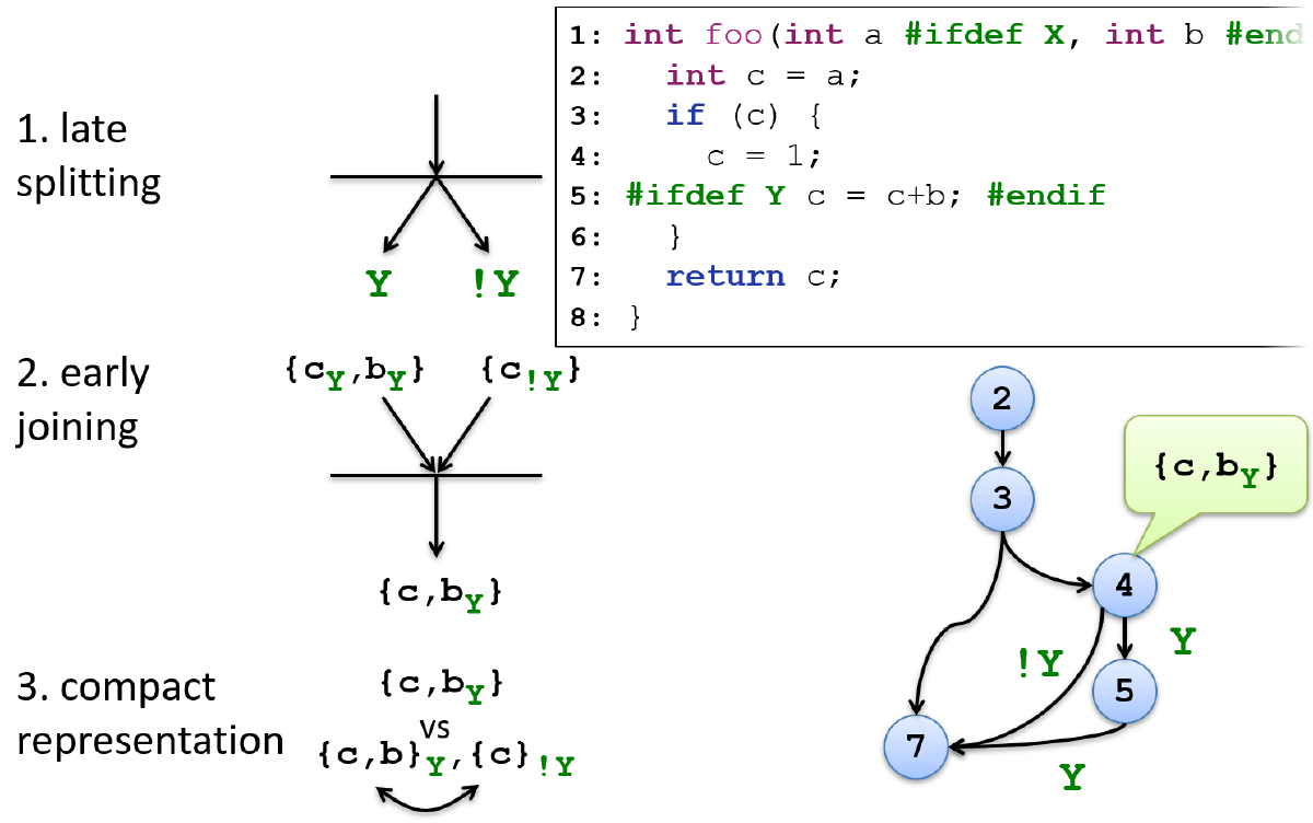
The following three principles ensure that analysis results are shared between different variants. The three principles are explained using the example of a variability-preserving Liveness analysis. Liveness is a classical data flow analysis that calculates for a concrete node in the CFG which variables are live, i.e. still used in the further program flow. The calculation of the live variables returns a set of variables. This quantity can be used for it, in order to determine conservatively Dead code (more exactly Dead Stores). Dead code represents program parts, which are not used and for optimization purposes can be deleted. In the concrete case the variable b is used only if the configuration option Y is switched on.

1. with the principle Late Splitting is ensured that an analysis does not run variability-true until variability in the input occurs. In the concrete example, the analysis splits with the variable control flow for the assignment c = 1. That is, the analysis is split and separate analysis results are calculated for the two paths Y and !Y. Thus, the result {cY,bY`` is obtained for path Y.

2. the principle of Early Joining ensures that results of different analysis paths are merged whenever commonalities in the input are reached. In the specific case, analysis paths computed by Late Splitting are joined into one overall result. In this process, variability information of the same paths is logically combined. Y and !Y become true by Y v !Y (with the logical or/v), because the variable c is live in both paths respectively.

3. the principle Compact Representation addresses the way analysis results are stored. In the figure, two different representations are shown for the result assembled under Principle 2. The first representation {c,bY} is more compact than the second one. Variability information is placed directly at the variables instead of result sets (like {c,b}Y). In our example, the effects are still small. However, if we assume that the variable c occurs in 2⁶⁰⁰⁰ different variants, then this variable would have to be stored just as frequently in different result sets, which is not possible in practice. That is, the first representation shows redundancy-free storage of the analysis results.

Outlook

Using these three principles, it could be shown for different analyses (including type checking, model checking and data flow analyses) that an astronomically large number of different variants can be analyzed efficiently. The actual analyses and additional efforts are thus reduced to a manageable number of variants and is thus also applicable to systems such as the Linux kernel. Thus, various questions can be answered for all variants that can be created by a configurable system.

The following papers describe further details of the implementation:

• Jörg Liebig, Alexander von Rhein, Christian Kästner, Jens Dörre, and Sven Apel. Scalable Analysis of Variable Software (European Software Engineering Conference and ACM SIGSOFT International Symposium on the Foundations of Software Engineering (ESEC/FSE)), pages 81-91, ACM Press.